Uncertainty and Reliability in the Eora MRIO tables

When you view the input-output tables or supply-use tables of countries of the Eora database you will notice many elements that are small and/or highly fluctuating between years. Naturally one might ask, what is the reliability and significance of such elements?

To understand this feature, let us recall that the estimation of any large multi-region input-output (MRIO) table such as the Eora database is an underdetermined problem. This means that the number of raw data items that can serve as support points for the most IO matrices is much smaller than the number of matrix elements. The estimation of a full IO table proceeds in a way that an initial estimate is constructed first, and then adjusted so that all elements conform as much as possible with the information contained in the raw data items.

This adjustment is generally carried out by using an optimisation algorithm. Such an algorithm is fed with three ingredients: A vectorised version P₀ of the initial estimate of the IO table, a vector c containing all raw data points, and a matrix G of constraints coefficients. The matrix G contains the relationships between the raw data points and the IO table elements; it has therefore as many rows as there are raw data points, and as many columns as there are IO table elements. The optimiser then adjusts P in order to reconcile G×P with the externally prescribed raw data c. In other words, the raw data c act as constraints on the vector P, and an optimal solution is found for P, that fulfils G×P = c as much as possible.

We call the vector G×P the constraint realisations, and we want these realisations to be equal to the actual constraints c as much as possible. In reality, there will generally not be a perfect match. This is because the set of constraints c contains raw data points with conflicting information. This happens, when different data sources provide different values for one and the same quantity.

During the optimisation, or matrix balancing process, elements that are supported by only few raw data, and hence restricted by only few constraints, can be subject to large adjustments, and hence their reliability is low. On the other hands, for virtually all large and important IO table elements, there exist supporting raw data, so that the adjustment of these elements is usually minimal, and hence their reliability is high. You can verify this feature in any of the many “hillside” (Fig. 1) or “rocket” graphs (Fig. 2) accessible from the data quality tabs. These will show that large transactions in the IO table (in vector notation, P) have a relatively small standard deviation and are relatively well constrained compared to smaller transactions.

The hillside diagrams show that relative standard deviations (sigma_rel) of the IO table P are small for large table elements, and vice versa (Fig. 1).

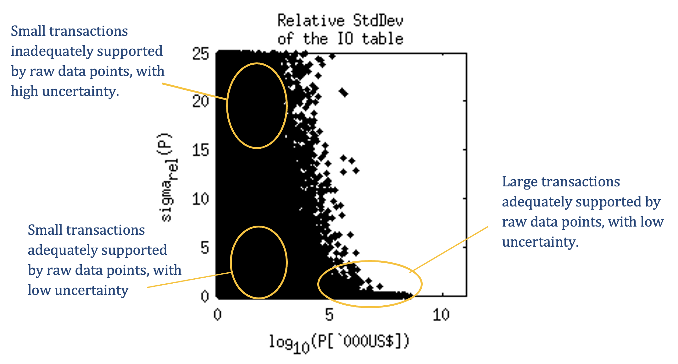
Figure 1 - The larger the value of transactions in the MRIO table (vectorized as P), the smaller the relative standard deviation sigma_rel.

Another way of looking at this issue is to consider the constraint realisations GP. Because the externally fixed raw data c conflict, the optimiser can generally not find a solution P where the realisations GP perfectly match all constraints c, it can only find a solution that is optimal in some defined sense. In other words, conflicting raw data will result in discrepancies between constraints c and their realisations GP. However, these discrepancies are only large for unimportant small elements (Fig. 2).

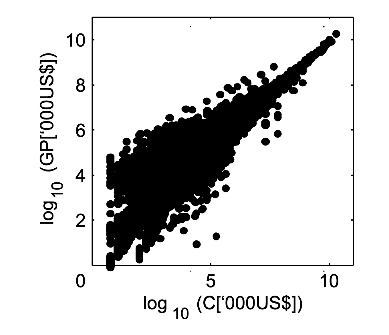
Figure 2 – Constraint realisations GP match constraints c more closely for large values. This figure shows the realizations for the USA in 2002.

There exists a well-known example problem arising out of conflicting information. Data on country-wise total exports and imports fundamentally conflict with global trade balances. One cannot achieve a balanced global multi-region input-output table whilst at the same time respecting data on exports and imports. This means that in a real MRIO table, either balancing conditions must be violated or raw data misrepresented. You can verify this in the current Eora tables that have been constructed with emphasis on a) representing large data items and b) fulfilling balancing conditions for large countries. For most countries, exports and imports are smaller than GDP, and in fact those exports and imports deviate somewhat from raw data given in the UN’s Main Aggregate database¹. For some countries such as Singapore and Hong Kong, exports and imports are larger than GDP, and for these countries, predominantly the GDP estimates deviate from raw data. Similarly, balancing conditions are usually very well met (1% imbalance) for large economies such as the USA, Japan, China and Germany, but less well met for small countries (up to 50% imbalance for example for São Tomé & Principe).

Confronted with these reliability issues, researchers have asked the following questions:

1. Does it make sense to construct IO tables at high detail if many of the ensuing elements are insufficiently supported by raw data?
2. Will the large number of small and unreliable elements lead to low-quality results for multipliers, footprints, and other impact measures?

With respect to the first question, one can show via Monte-Carlo simulation that it is always beneficial for IO table construction to use as much information as possible. Choosing to aggregate the table’s sector classification even when only one disaggregated raw data item were available would mean losing information. Also, even if we were only interested in an aggregated final table, it would be better to construct a disaggregated table first, undertake the multiplier or footprint analysis, and then aggregate the results. For further information on this issue see ² and references therein.

Regarding the second question, Jensen ³ has demonstrated that a large number of small elements can be perturbed without significantly changing estimates for multipliers or footprints. Jensen and West ³ report that a surprisingly large number of smaller elements in an IO table can even be removed before multipliers show a significant change, because the value of these elements is often negligible compared to the combined value of a few large elements. Since Jensen’s pioneering work, this phenomenon has become known as holistic accuracy. While table accuracy represents the conventional understanding of the accuracy of single matrix elements, holistic accuracy is concerned with the representativeness of a table of the synergistic characteristics of an economy. In this perspective, the accuracy of single elements may be unimportant, as long as the results of modeling exercises yield a realistic picture for the purpose of the analyst or decision-maker. In other words, unless someone is actually interested in single table elements as such, it does not matter to have a large number of small and unreliable elements in an IO table.

This means that users of the Eora tables should view all quantitative information in light of their varying degree of reliability, and make use of the information provided only within the bounds of its statistical significance. The Eora team believes that it is beneficial to provide IO data as values along with their standard deviations, so that decision-makers can judge any quantitative information not only with respect to its magnitude, but also with regard to its reliability. For example, analysts may choose to aggregate the Eora database into a format that is more suitable for their purposes, and in this case Eora’s accompanying standard deviation matrices provide all that is needed to calculate the standard deviations of any aggregated table, using standard error propagation.

The method used in the Eora tables for determining MRIO standard deviations is described in ⁵. In essence, this method fits an error propagation formula to the standard deviations of raw data that are used for constructing the tables. Such standard deviations can in most cases only be guessed, since very little information is available on the uncertainty of macroeconomic and input-output data. Hence, the standard deviations of raw data, and as a consequence also the standard deviations of the MRIO table elements, are based on assumptions, or choices. The Eora tables as published were estimated assuming that national input-output tables were most reliable, with the narrowest standard deviation settings, followed by UN Main Aggregates and Official Country data ^{1, 6} (for years where national input-output data do not exist), and then followed by UN Comtrade data⁷. The latter were considered least reliable, partly because of severe conflict and errors that have previously been identified also by other research teams ⁸. As a result, a set of Eora tables should be viewed as based on a particular world view of uncertainty, or reliability. For other world views, one could re-specify standard deviations, and re-run the Eora construction routines. One would then obtain a different set of tables. Hence, there is no one unique set of MRIO tables.

References

1. UNSD. National Accounts Main Aggregates Database. Report No. http://unstats.un.org/unsd/snaama/Introduction.asp, (United Nations Statistics Division, New York, USA, 2011).
2. Lenzen, M. Aggregation versus disaggregation in input-output analysis of the environment. Economic Systems Research 23, 73 – 89 (2011).
3. Jensen, R. C. The concept of accuracy in regional input-output models. International Regional Science Review 5, 139-154 (1980).
4. Jensen, R. C. & West, G. R. The effect of relative coefficient size on input-output multipliers. Environment and Planning A 12, 659-670 (1980).
5. Lenzen, M., Wood, R. & Wiedmann, T. Uncertainty analysis for Multi-Region Input-Output models – a case study of the UK’s carbon footprint. Economic Systems Research 22, 43-63 (2010).
6. UNSD. National Accounts Official Data. Report No. data.un.org/Browse.aspx?d=SNA, (United Nations Statistics Division, New York, USA, 2011).
7. UN. UN comtrade - United Nations Commodity Trade Statistics Database. Report No. comtrade.un.org/, (United Nations Statistics Division, UNSD, New York, USA, 2011).
8. Oosterhaven, J., Stelder, D. & Inomata, S. Estimating international interindustry linkages: non-survey simulations of the Asian-Pacific economy. Economic Systems Research 20, 395-414 (2008).